Self-Driving RC Car
Ivan Oršolić - Master's Thesis.
Why a self-driving RC car?
🛈 Video source: Waymo, Sensor VisualizationWhat to look for in an RC car?
-
📐 Scale
-
🏎️ Body type
-
⚙️ Electric motor type
-
🦾 Steering servo
-
🚥 Electronic Speed Controller
-
⚡🔋 Batteries
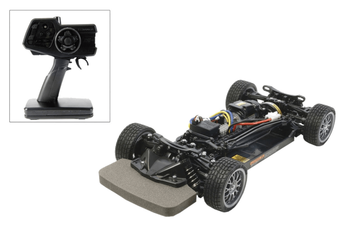
Bill of materials
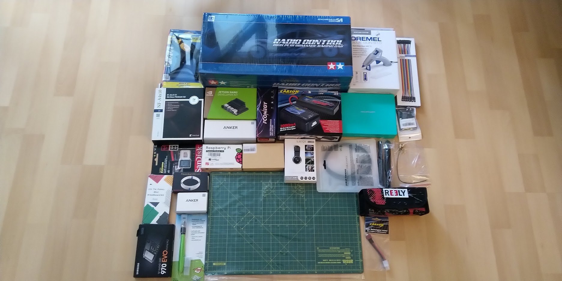
An RC car
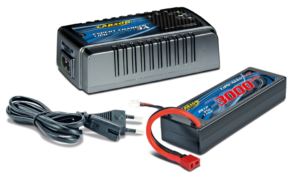
Charger and batteries
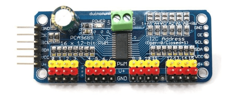
A PWM/Servo Driver (I2C + some jumper cables)
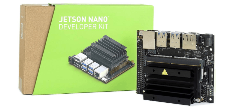
A Jetson Nano
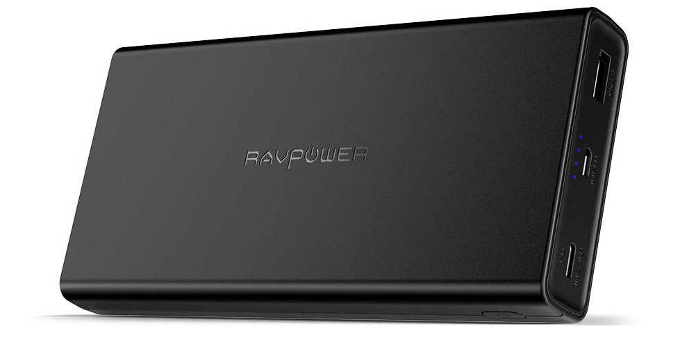
A powerbank (+ some usb cables)
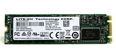
A microSD card (and optionally an external SSD)
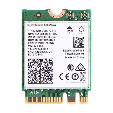
A WiFi/BT m.2 card (key E) or some USB equivalent
A camera

–
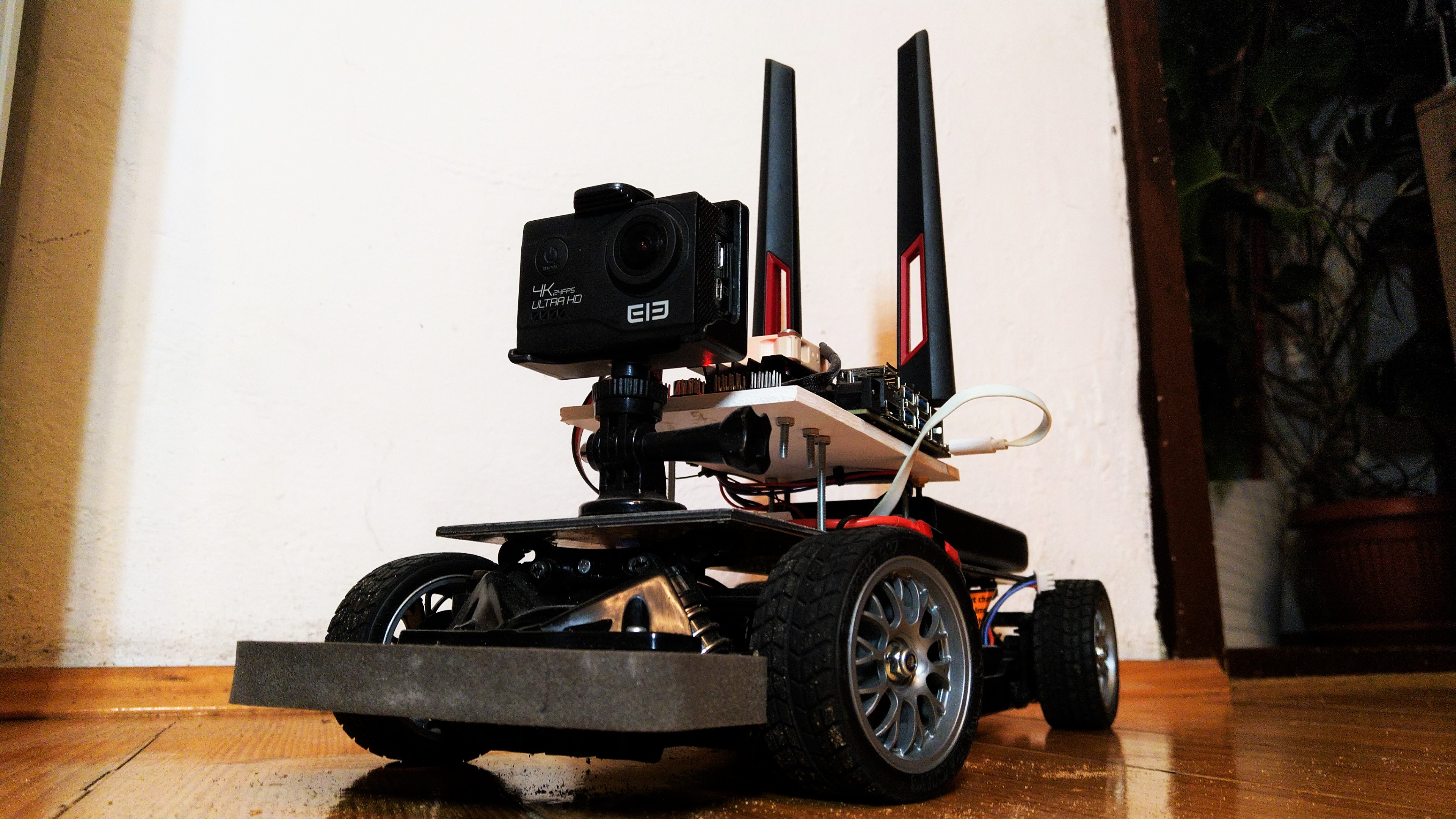
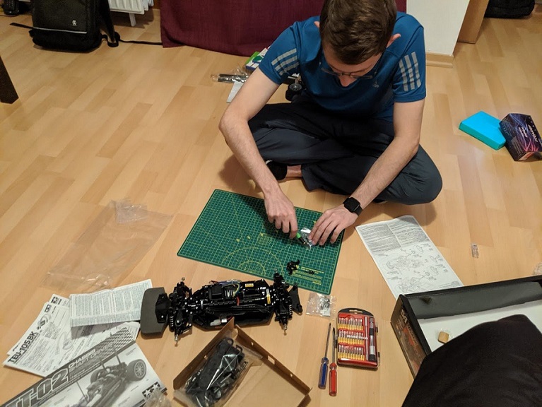
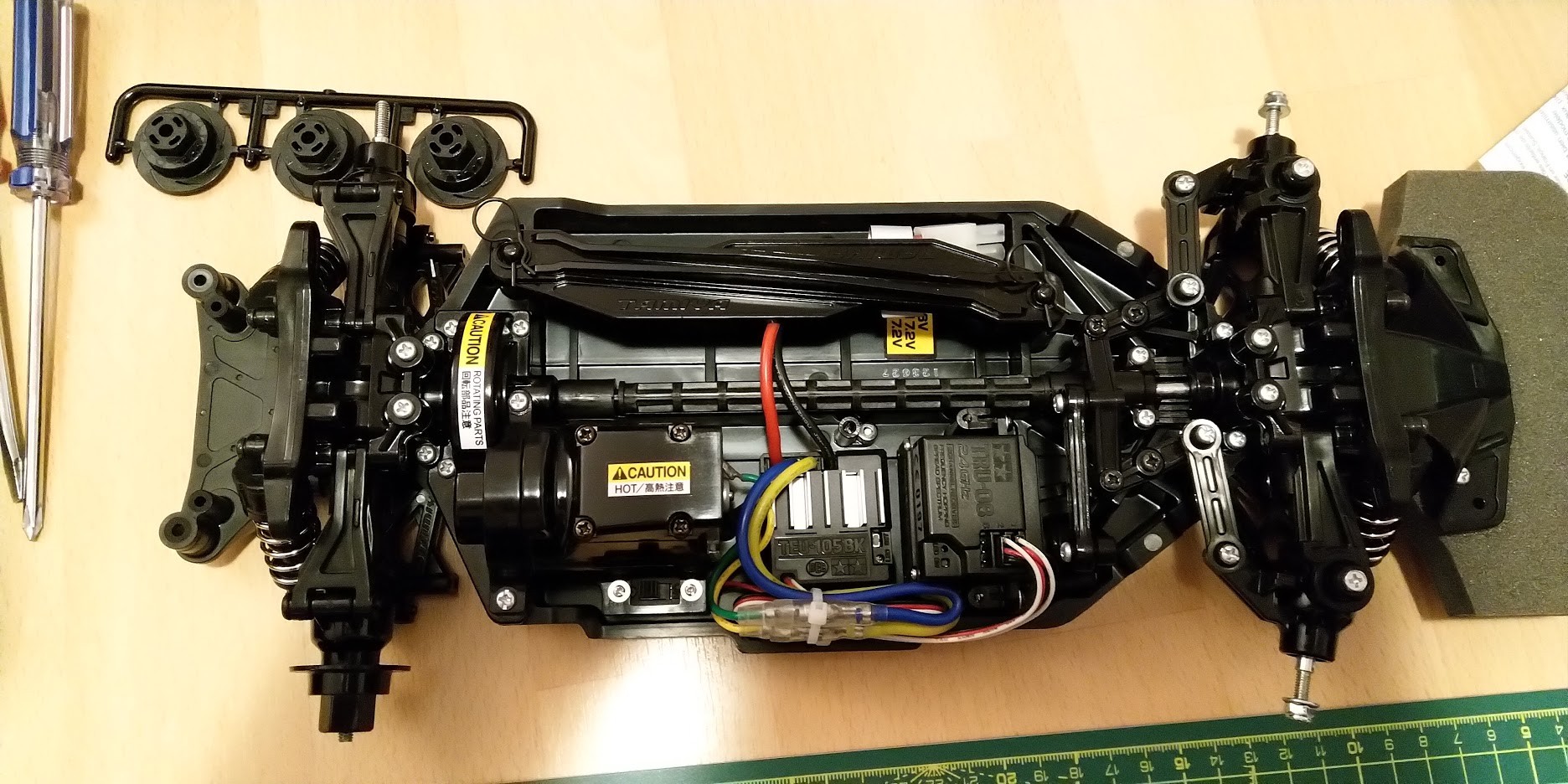
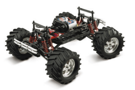
Assembling the RC car
RTR Kit
Wheel base
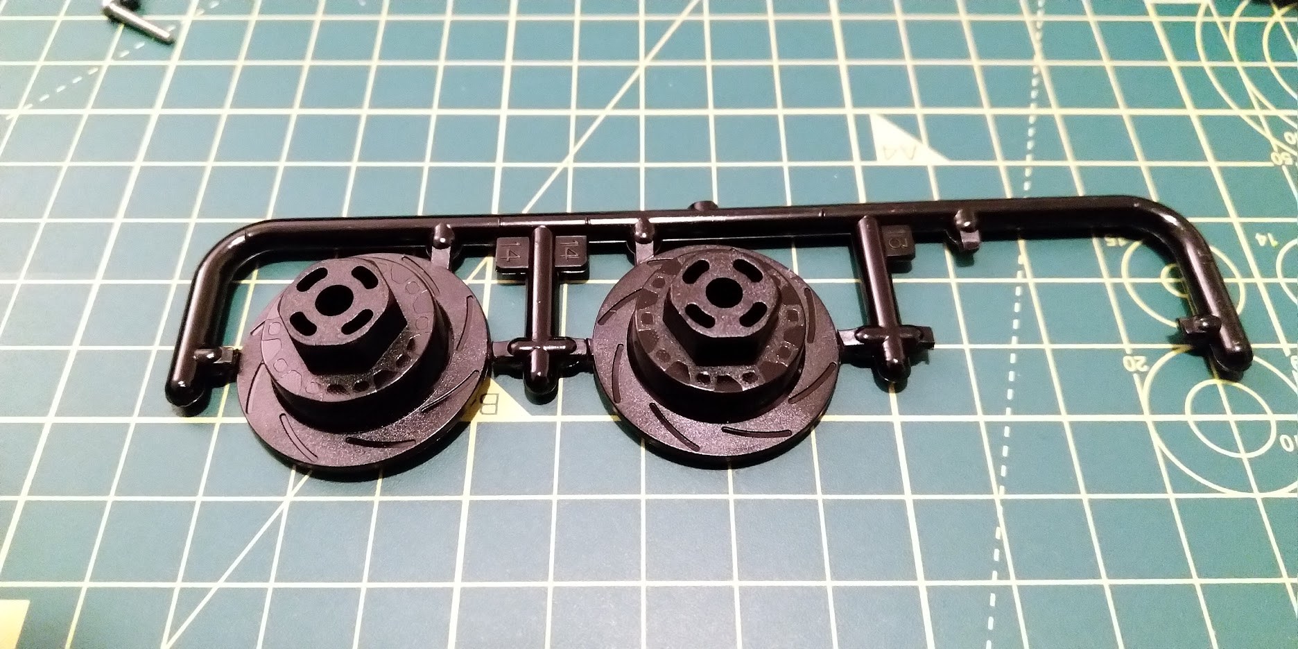
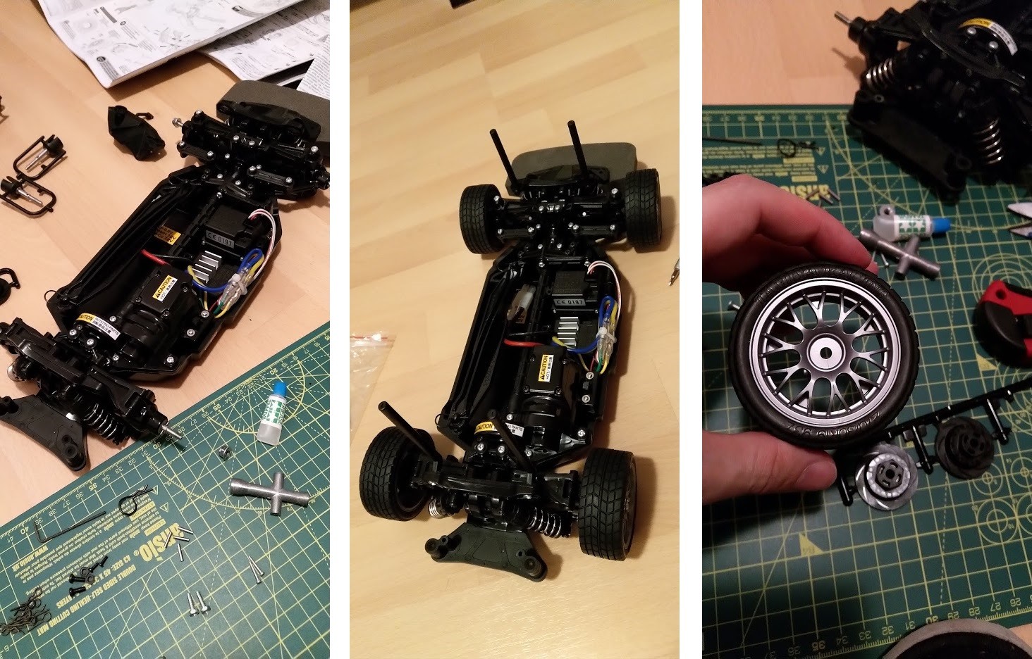
Mounting the wheels
Mounting the wheels
Assembling the mounting plates
Option 1: 3D Printed parts
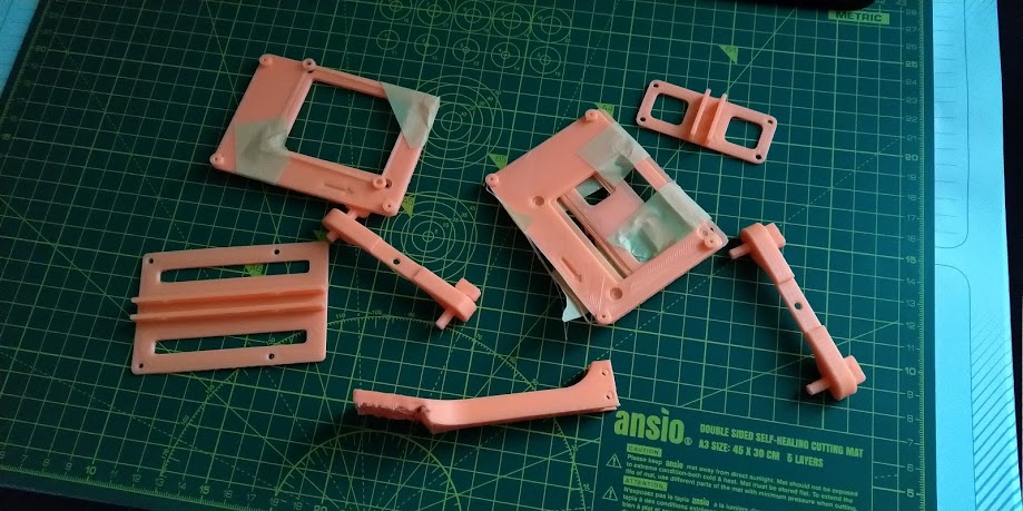
Option 2: Custom made mounting plates
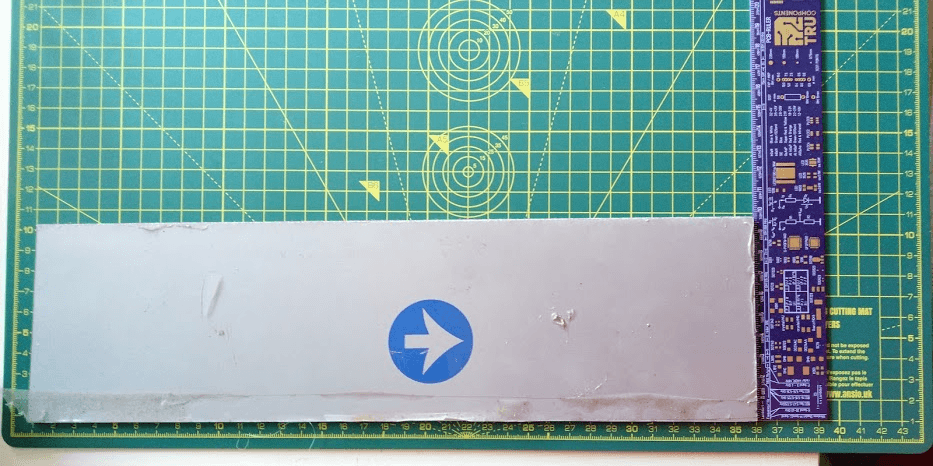
3D model of the custom mounting plates
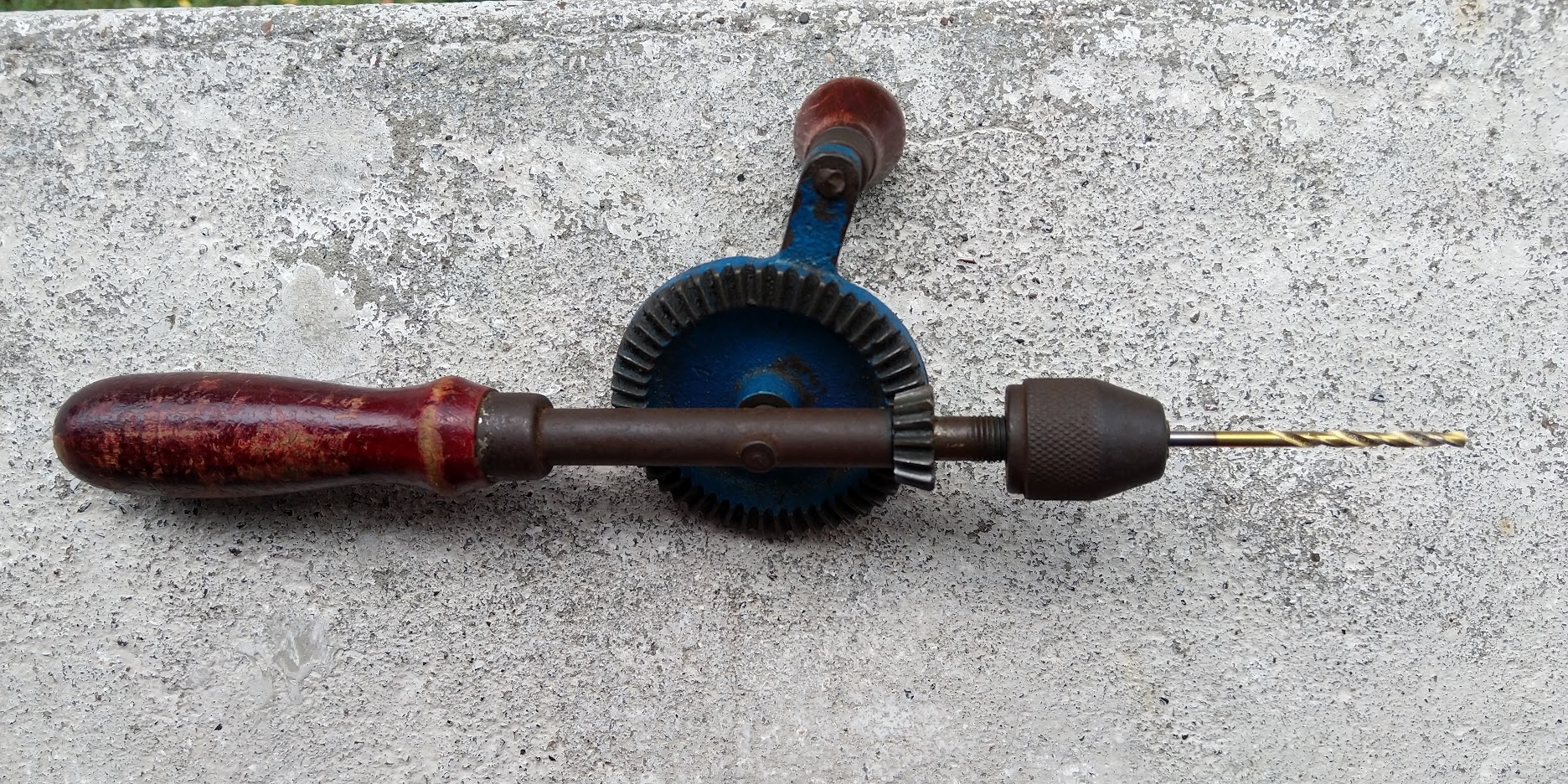
Power tools
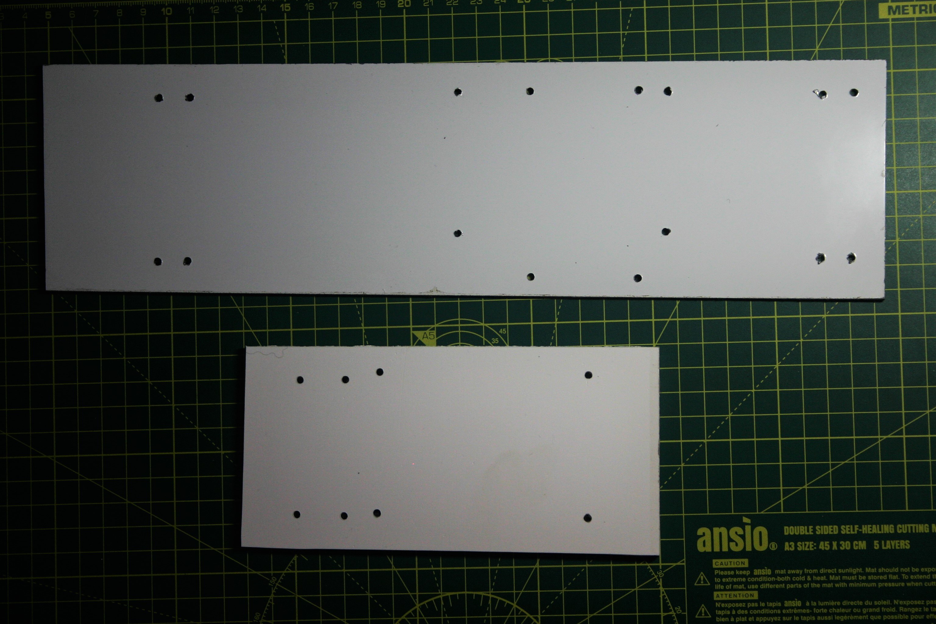
Drilled mounting plates
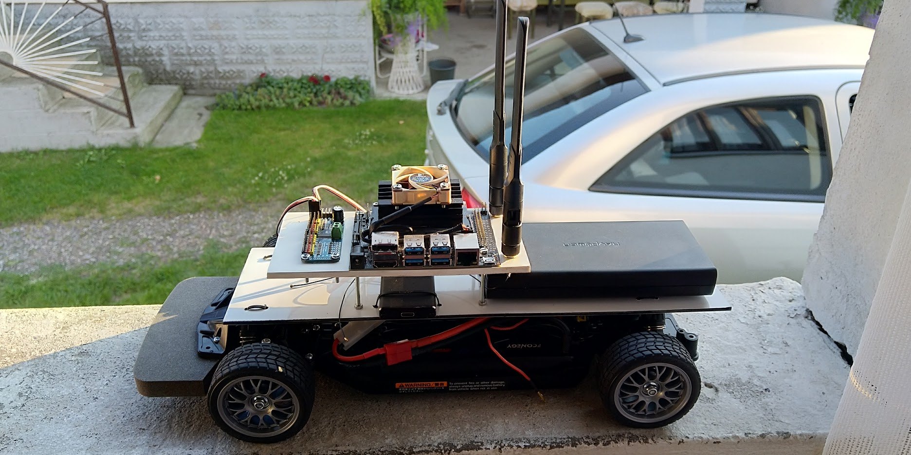
(Semi) Finished car
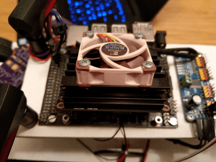
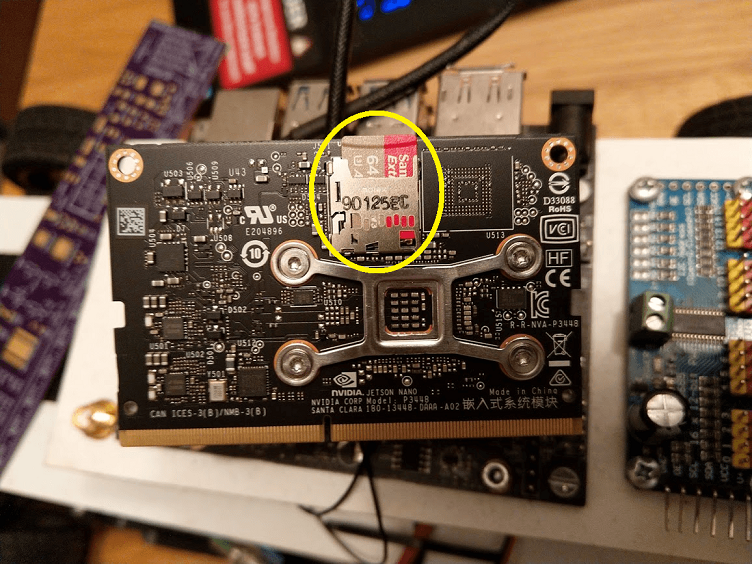
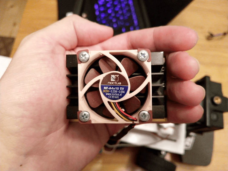
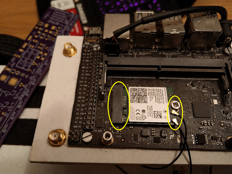
Jetson Nano assembly
Taking out the Nano module
MicroSD slot
Adding the fan
Adding the WLAN/BT card
Connecting the RC car to the Jetson Nano
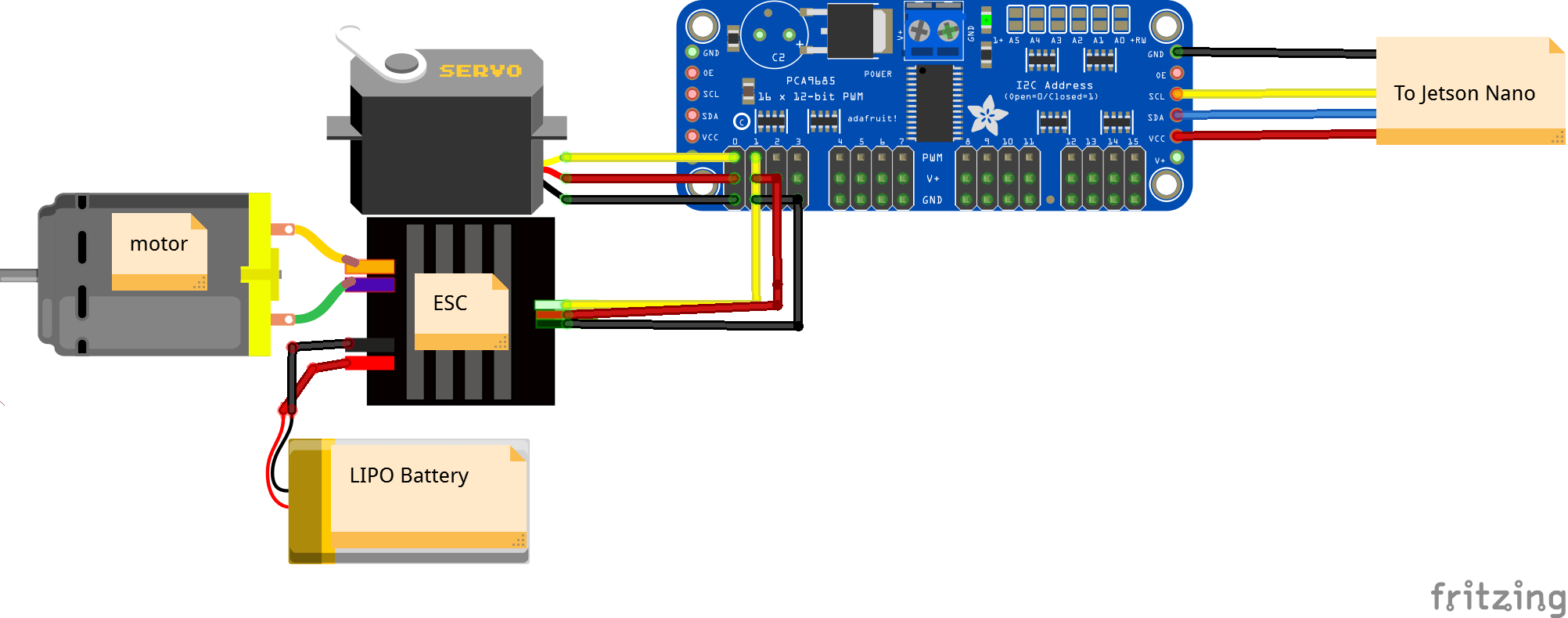
The schematic
Finding the ESC/Servo
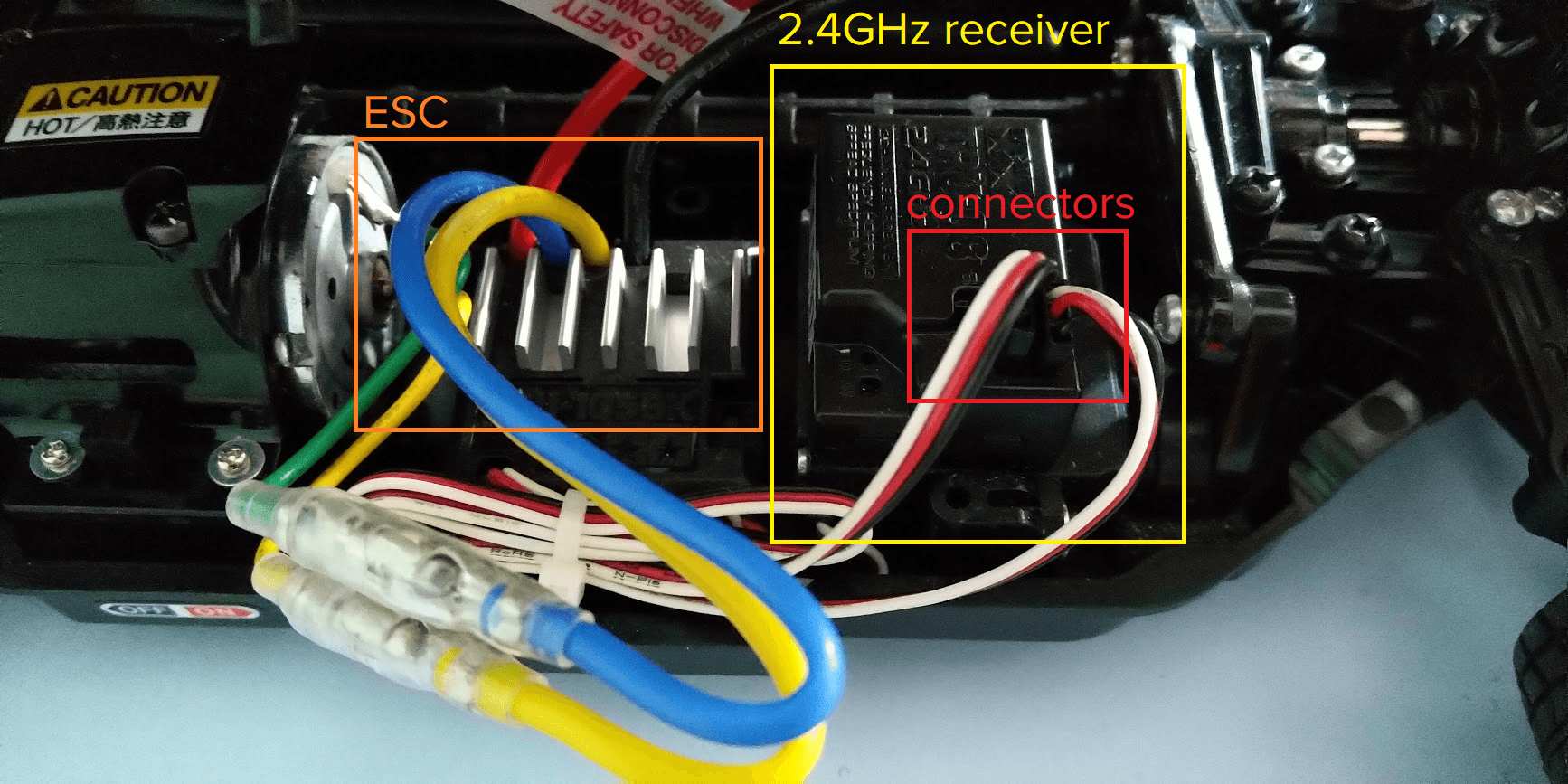
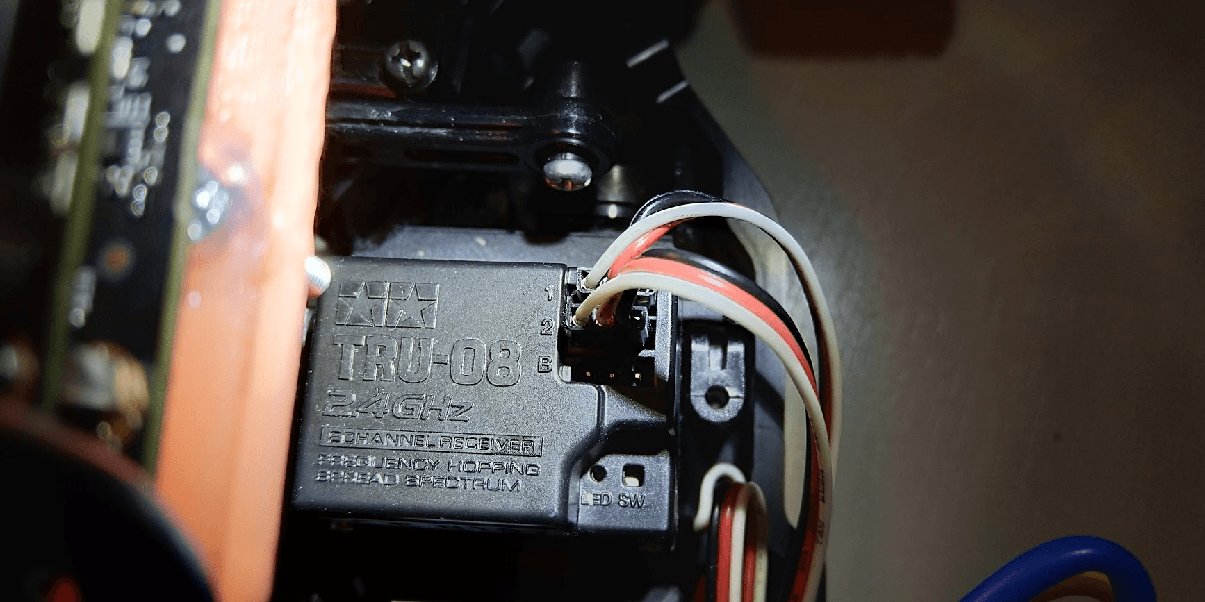
Wireless receiver
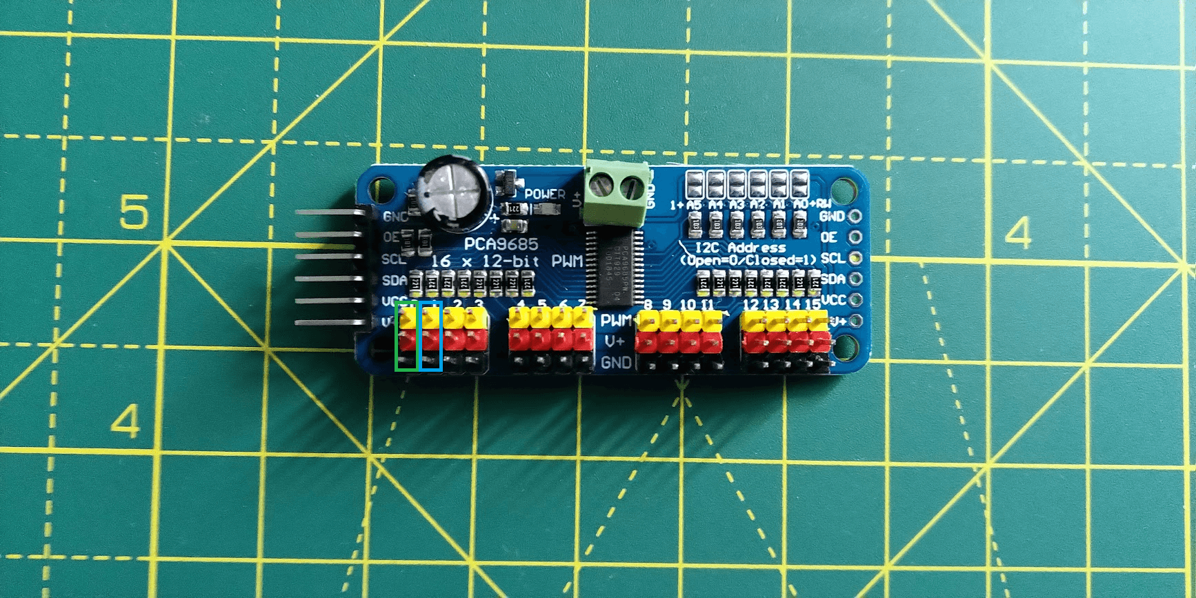
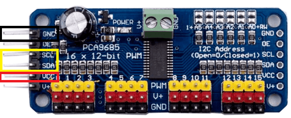
PCA9685
ESC -> PCA9685
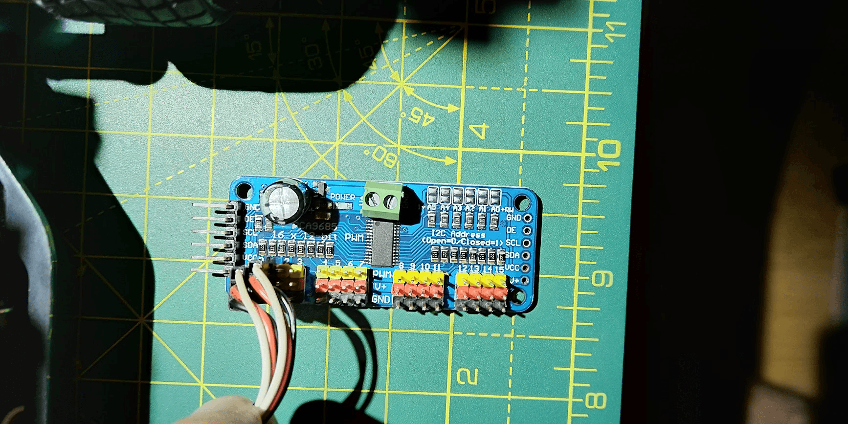
PCA9682 I2C Port
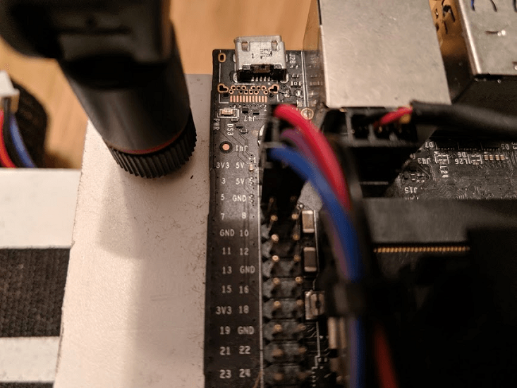
Jetson Nano I2C Pins
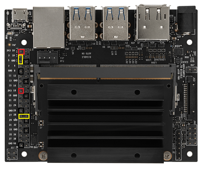
PCA9685 -> Jetson Nano
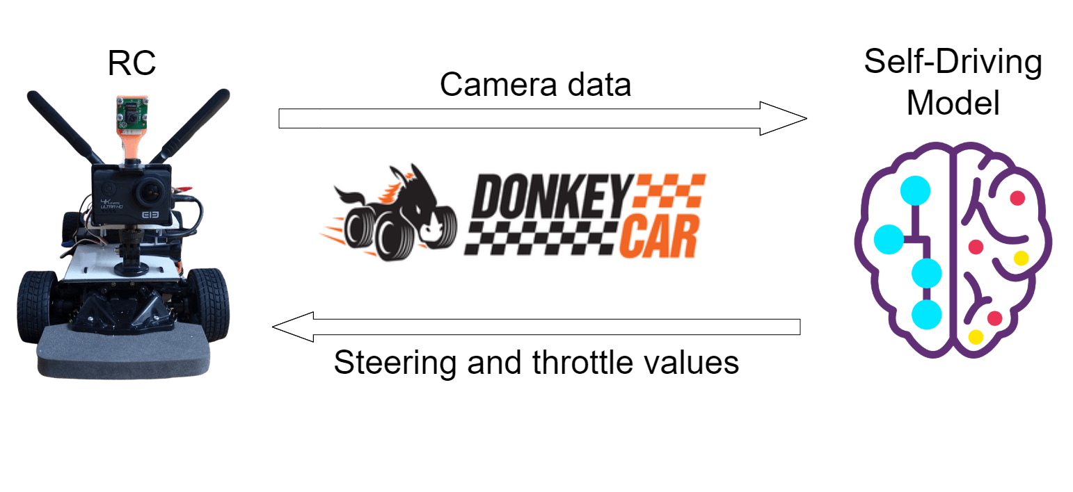
DonkeyCar
What is Donkey?
Donkey is a high level self driving library written in Python.
How was it used?
It was used as an interface between the RC car and the neural net that controls the car.
Things Donkey solves:
-
📷Data preprocessing
-
🎮Controlling the RC car
-
✅Data collection/labeling
-
🏋️♂️Custom model training
-
Question: RC Car only or Host PC + RC ❓
Donkey RC calibration
Steering calibration
Throttle calibration
Gamepad steering
Gamepad Throttle
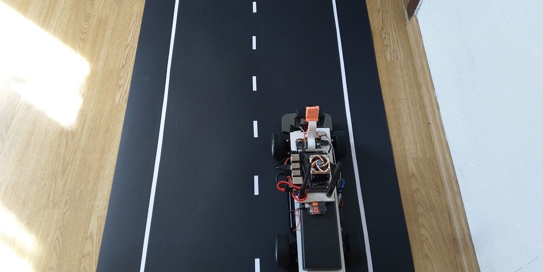
Sanity check
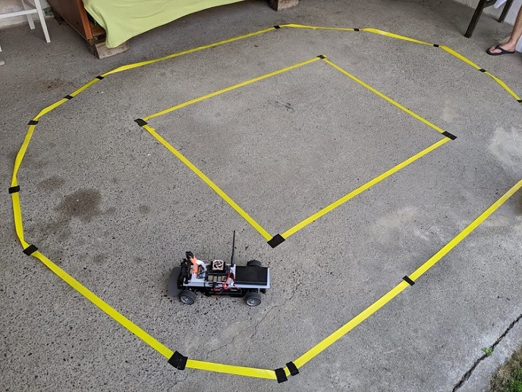
First test track
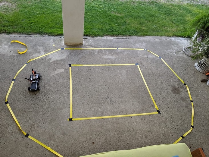
Fancier test track
Collecting training data
First basic autopilot
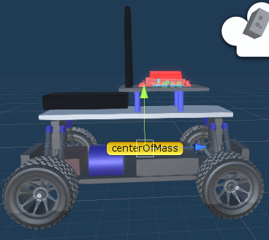
Custom simulator
Why use a simulator?
Pretty simple: rapid prototyping in a safe and reproducible environment.
💡 Fun fact: Tesla spends a lot of time and money on their simulator.
Caveat emptor:
Real data has no substitutes.
What makes a good sim
Image resolution
Real-world fidelity
Physics? Model translation?
DARPA Grand Challenge 2004
First neural network
Dave
(DARPA Autonomous Vehicle)
An RC Car with two cameras autonomously driving through a junk-filled alley way.
DAVE-2 Architecture
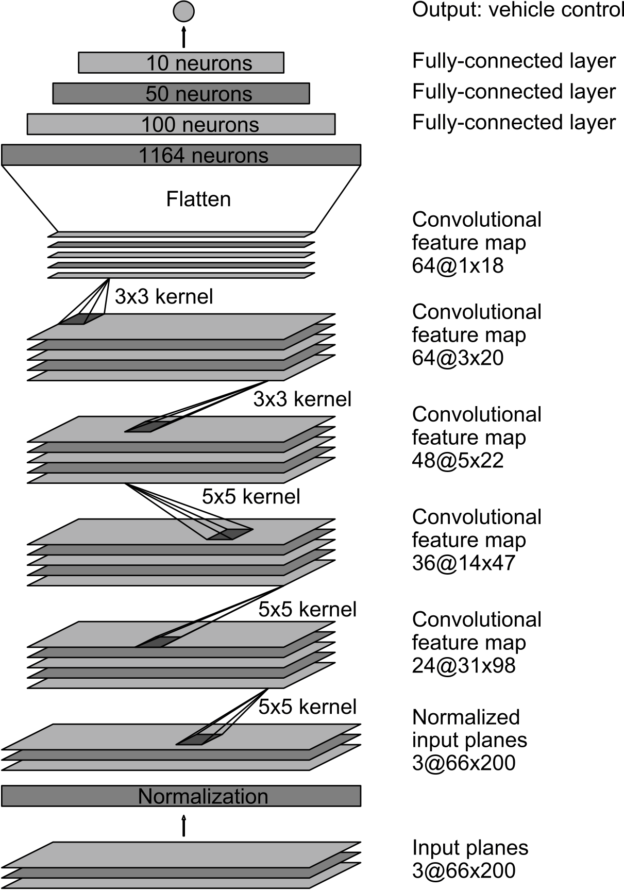
Slight adjustions made:
-
✂ Omitted the normalization layer for now.
-
➕Added a 25 unit and a 5 unit layer.
-
💤 Added dropout regularization (90%).
-
🚙💨Two output units for steering and throttle.
Implementing the DAVE-2 network
Keras model
def customArchitecture(num_outputs, input_shape, roi_crop):

    input_shape = adjust_input_shape(input_shape, roi_crop)
    img_in = Input(shape=input_shape, name='img_in')
    x = img_in

    # Dropout rate
    keep_prob = 0.9
    rate = 1 - keep_prob

    # Convolutional Layer 1
    x = Convolution2D(filters=24, kernel_size=5, strides=(2, 2), input_shape = input_shape)(x)
    x = Dropout(rate)(x)

    # Convolutional Layer 2
    x = Convolution2D(filters=36, kernel_size=5, strides=(2, 2), activation='relu')(x)
    x = Dropout(rate)(x)

    # Convolutional Layer 3
    x = Convolution2D(filters=48, kernel_size=5, strides=(2, 2), activation='relu')(x)
    x = Dropout(rate)(x)

    # Convolutional Layer 4
    x = Convolution2D(filters=64, kernel_size=3, strides=(1, 1), activation='relu')(x)
    x = Dropout(rate)(x)

    # Convolutional Layer 5
    x = Convolution2D(filters=64, kernel_size=3, strides=(1, 1), activation='relu')(x)
    x = Dropout(rate)(x)

    # Flatten Layers
    x = Flatten()(x)

    # Fully Connected Layer 1
    x = Dense(100, activation='relu')(x)

    # Fully Connected Layer 2
    x = Dense(50, activation='relu')(x)

    # Fully Connected Layer 3
    x = Dense(25, activation='relu')(x)

    # Fully Connected Layer 4
    x = Dense(10, activation='relu')(x)

    # Fully Connected Layer 5
    x = Dense(5, activation='relu')(x)
    outputs = []

    for i in range(num_outputs):
        # Output layer
        outputs.append(Dense(1, activation='linear', name='n_outputs' + str(i))(x))

    model = Model(inputs=[img_in], outputs=outputs)

    return model
Using the model in Donkey
class NvidiaModel(KerasPilot):
    def __init__(self, num_outputs=2, input_shape=(120,160,3), roi_crop=(0,0), *args, **kwargs):
        super(NvidiaModel, self).__init__(*args, **kwargs)
        self.model = customArchitecture(num_outputs, input_shape, roi_crop)
        self.compile()

    def compile(self):
        self.model.compile(optimizer="adam",
                loss='mse')

    def run(self, img_arr):
        img_arr = img_arr.reshape((1,) + img_arr.shape)
        outputs = self.model.predict(img_arr)
        steering = outputs[0]
        throttle = outputs[1]
        return steering[0][0], throttle[0][0]
Test drive
Visualization
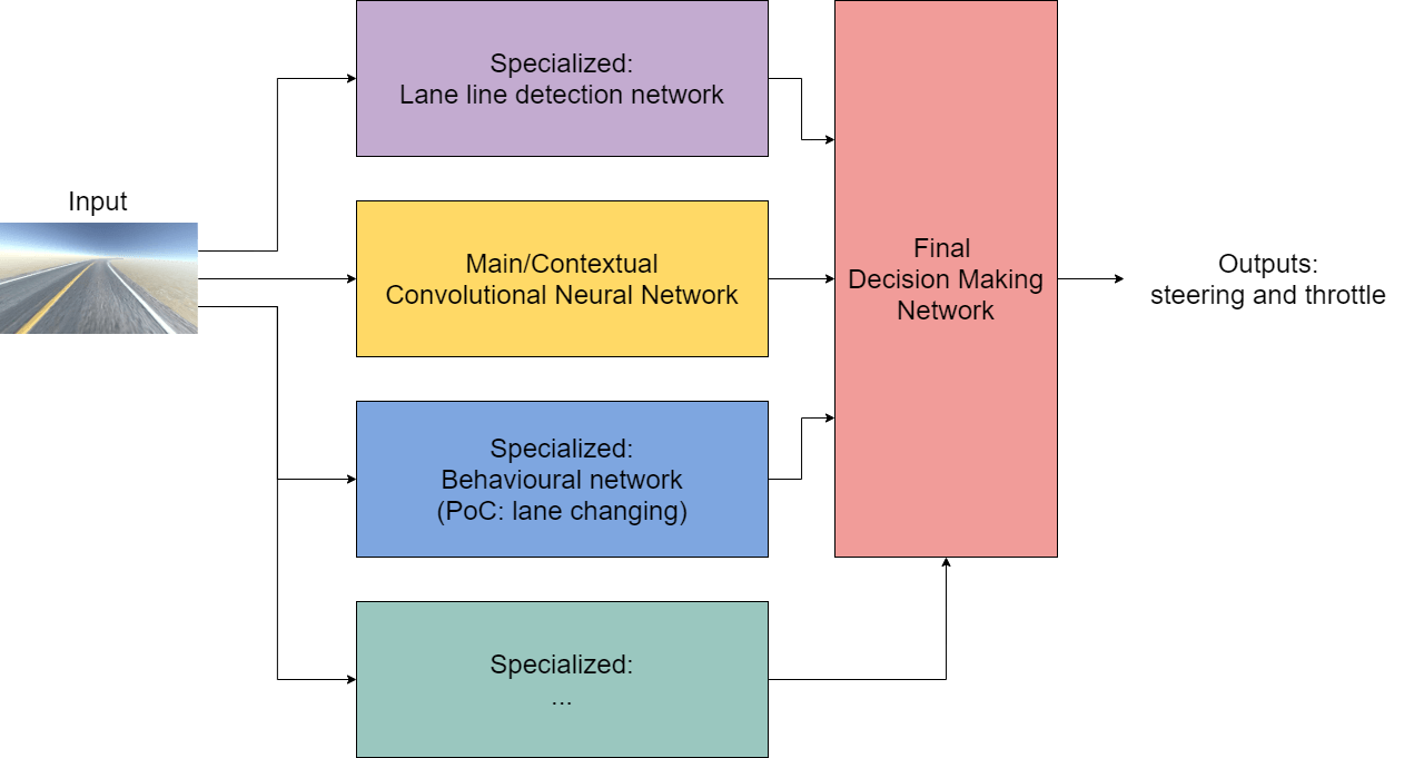
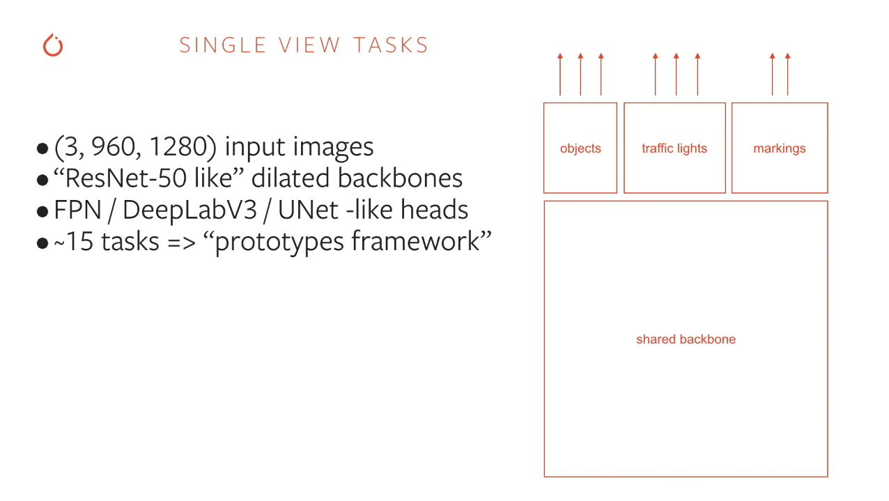
Architecture proposal
“Hydra”-like nets
Tesla's similar nets
First iteration
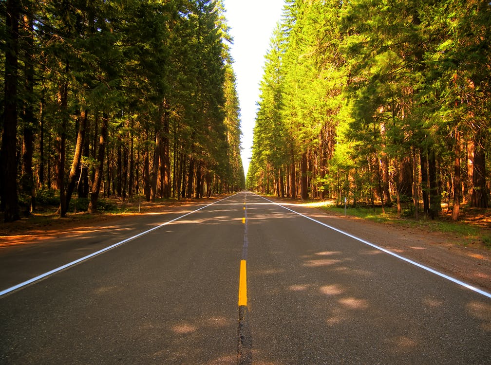
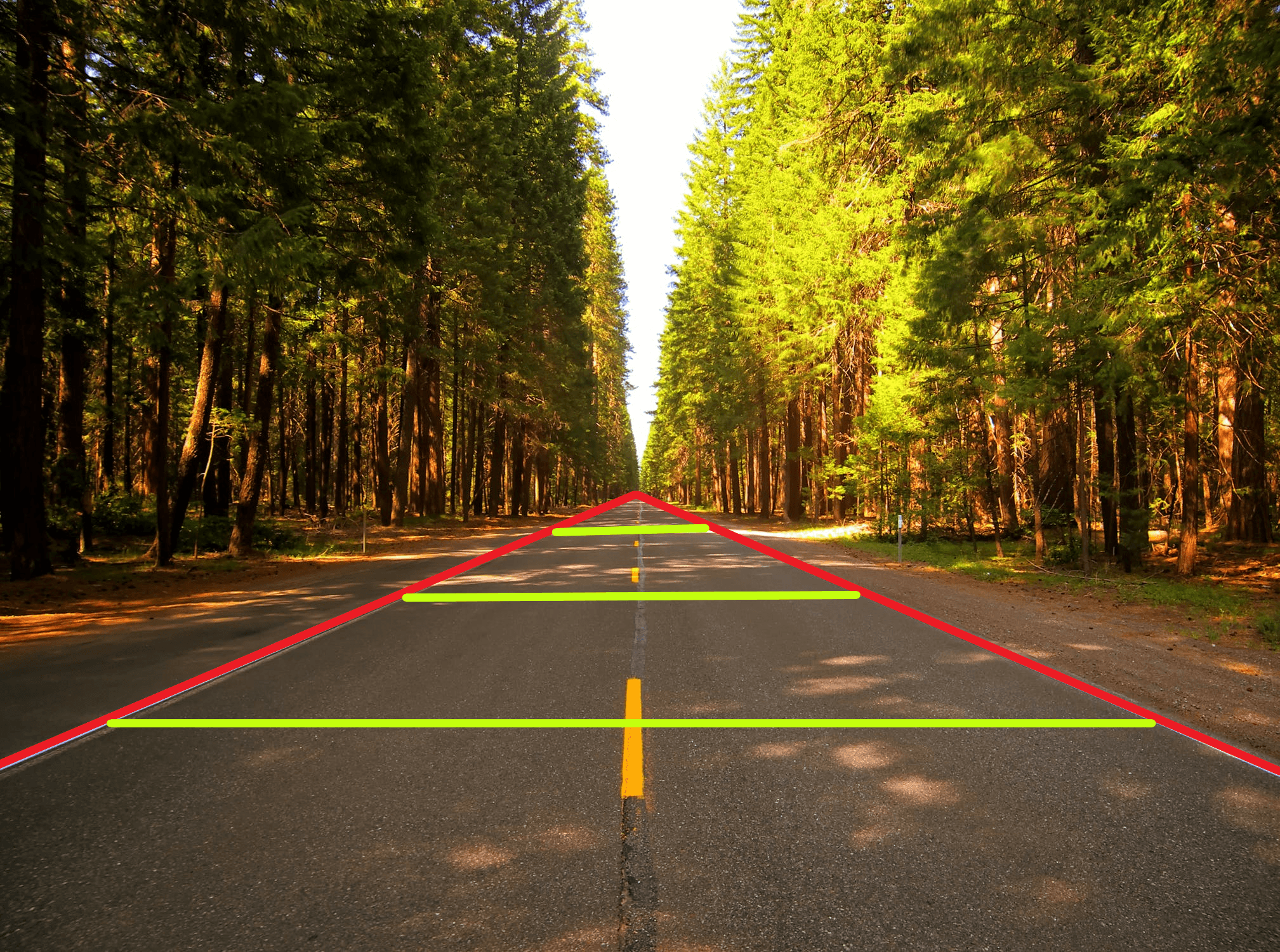
Lane extraction
Mapping the 3D world to 2D
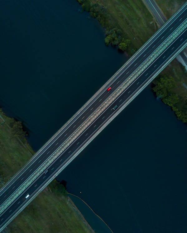
Parallel?
Another example
Parallel?
Train dronez?
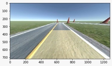
Warping the perspective

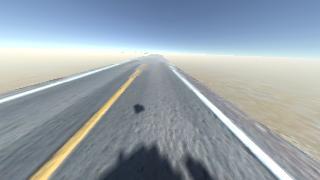
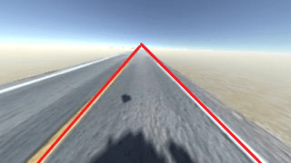
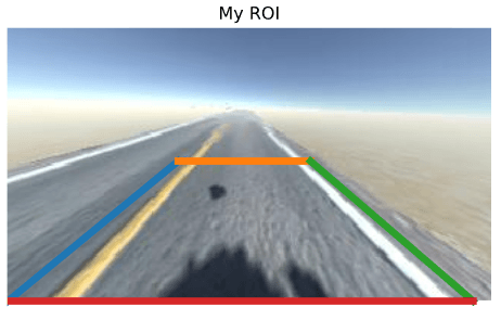
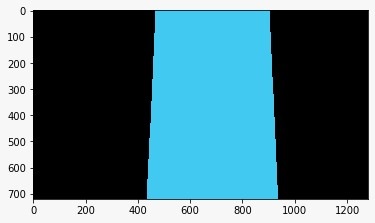
First step: ROI
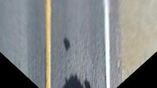
Second step: target perspective
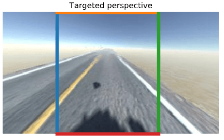
Final step: transform
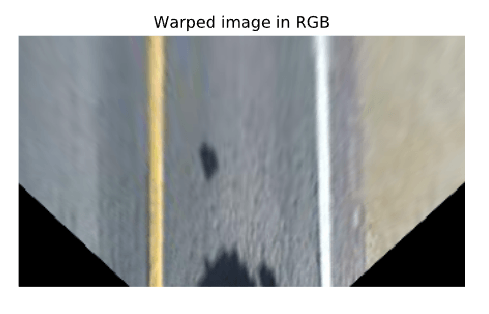
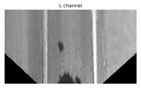
Making the lines easier to see
Converting to HSL color space
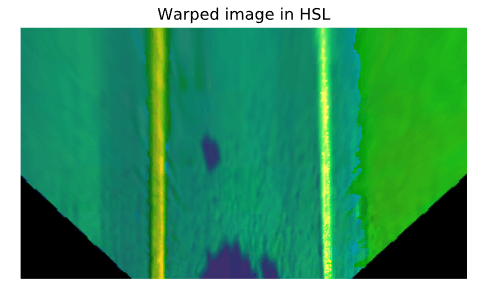
Split into separate channels
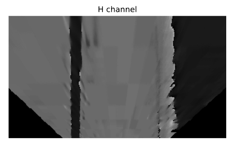
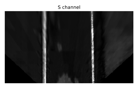
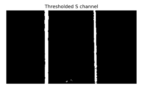
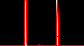
Threshold the S-channel
The entire process
Going one step further?
Fitting lanes using a polynomial approximation
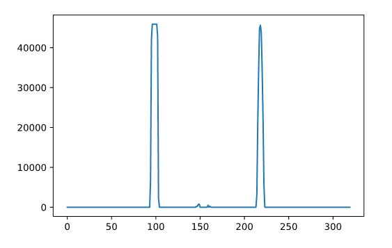
Histogram overlay
Found lane using polynomial fit
Unwarped image with detected lane
Polynomial fit in action
Why not to use it?
Implementing the lane finding
def warpImage(self, image):
    # Define the region of the image we're interested in transforming
    regionOfInterest = np.float32(
    [[0,  180],  # Bottom left
    [112.5, 87.5], # Top left
    [200, 87.5], # Top right
    [307.5, 180]]) # Bottom right

    # Define the destination coordinates for the perspective transform
    newPerspective = np.float32(
    [[80,  180],  # Bottom left
    [80,    0.25],  # Top left
    [230,   0.25],  # Top right
    [230, 180]]) # Bottom right
    # Compute the matrix that transforms the perspective
    transformMatrix = cv2.getPerspectiveTransform(regionOfInterest, newPerspective)
    # Warp the perspective - image.shape[:2] takes the height, width, [::-1] inverses it to width, height
    warpedImage = cv2.warpPerspective(image, transformMatrix, image.shape[:2][::-1], flags=cv2.INTER_LINEAR)
    return warpedImage

def extractLaneLinesFromSChannel(self, warpedImage):
    # Convert to HSL
    hslImage = cv2.cvtColor(warpedImage, cv2.COLOR_BGR2HLS)
    # Split the image into three variables by the channels
    hChannel, lChannel, sChannel = cv2.split(hslImage)
    # Threshold the S channel image to select only the lines
    lowerThreshold = 65
    higherThreshold = 255
    # Threshold the image, keeping only the pixels/values that are between lower and higher threshold
    returnValue, binaryThresholdedImage = cv2.threshold(sChannel,lowerThreshold,higherThreshold,cv2.THRESH_BINARY)
    # Since this is a binary image, we'll convert it to a 3-channel image so OpenCV can use it
    thresholdedImage = cv2.cvtColor(binaryThresholdedImage, cv2.COLOR_GRAY2RGB)
    return thresholdedImage

def processImage(self, image):
    warpedImage = self.warpImage(image)
    # We'll normalize it just to make sure it's between 0-255 before thresholding
    warpedImage = cv2.normalize(warpedImage,None,0,255,cv2.NORM_MINMAX,cv2.CV_8U)
    thresholdedImage = self.extractLaneLinesFromSChannel(warpedImage)
    one_byte_scale = 1.0 / 255.0
    # To make sure it's between 0-1 for the model
    return np.array(thresholdedImage).astype(np.float32) * one_byte_scale
Implementing the first iteration model
Model definition
def oriModel(inputShape, numberOfBehaviourInputs):

    # Dropout rate
    keep_prob = 0.9
    rate = 1 - keep_prob

    # Input layers
    imageInput = Input(shape=inputShape, name='imageInput')
    laneInput = Input(shape=inputShape, name='laneInput')
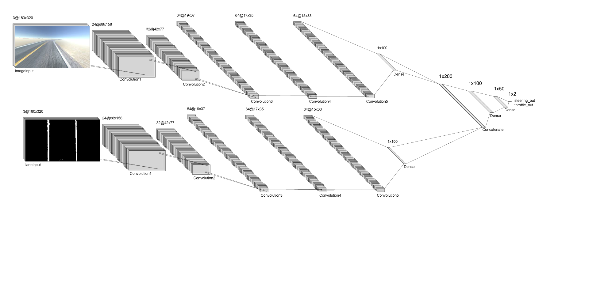
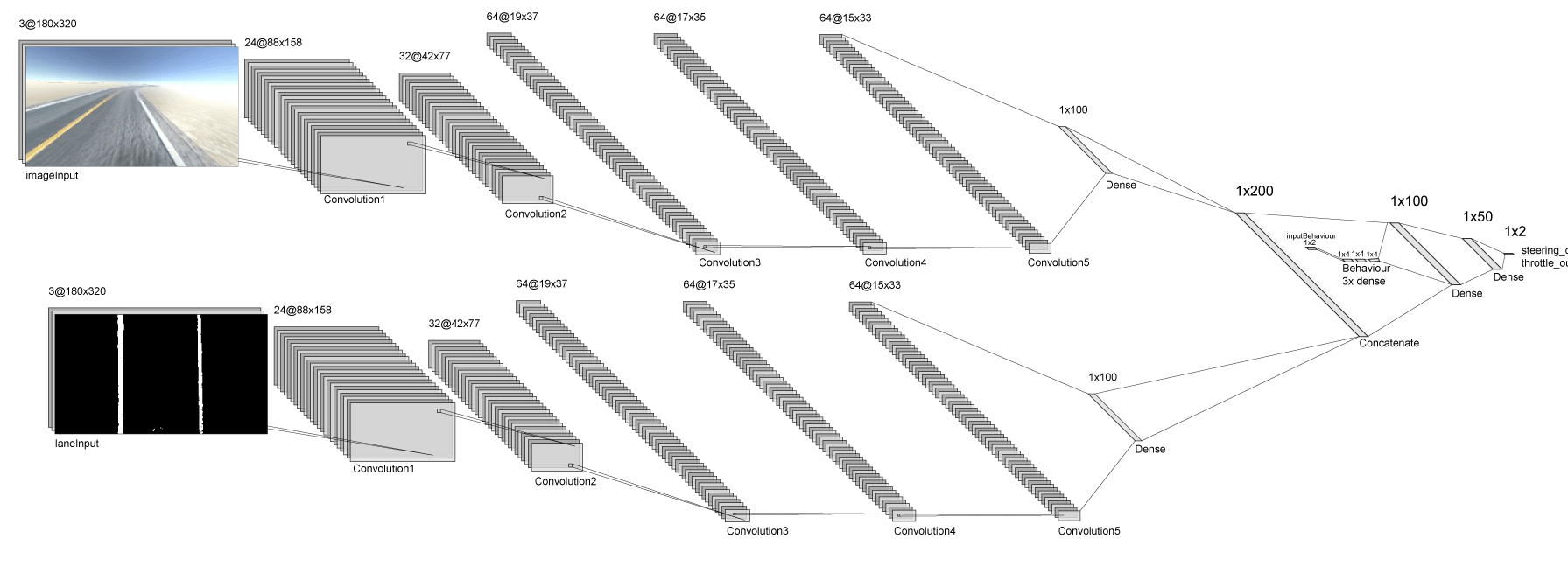
Generalized CNN
# Input image convnet
    x = imageInput
    x = Conv2D(24, (5,5), strides=(2,2), name="Conv2D_imageInput_1")(x)
    x = LeakyReLU()(x)
    x = Dropout(rate)(x)
    x = Conv2D(32, (5,5), strides=(2,2), name="Conv2D_imageInput_2")(x)
    x = LeakyReLU()(x)
    x = Dropout(rate)(x)
    x = Conv2D(64, (5,5), strides=(2,2), name="Conv2D_imageInput_3")(x)
    x = LeakyReLU()(x)
    x = Dropout(rate)(x)
    x = Conv2D(64, (3,3), strides=(1,1), name="Conv2D_imageInput_4")(x)
    x = LeakyReLU()(x)
    x = Dropout(rate)(x)
    x = Conv2D(64, (3,3), strides=(1,1), name="Conv2D_imageInput_5")(x)
    x = LeakyReLU()(x)
    x = Dropout(rate)(x)
    x = Flatten(name="flattenedx")(x)
    x = Dense(100)(x)
    x = Dropout(rate)(x)
Lane finding CNN
# Preprocessed lane image input convnet
    y = laneInput
    y = Conv2D(24, (5,5), strides=(2,2), name="Conv2D_laneInput_1")(y)
    y = LeakyReLU()(y)
    y = Dropout(rate)(y)
    y = Conv2D(32, (5,5), strides=(2,2), name="Conv2D_laneInput_2")(y)
    y = LeakyReLU()(y)
    y = Dropout(rate)(y)
    y = Conv2D(64, (5,5), strides=(2,2), name="Conv2D_laneInput_3")(y)
    y = LeakyReLU()(y)
    y = Dropout(rate)(y)
    y = Conv2D(64, (3,3), strides=(1,1), name="Conv2D_laneInput_4")(y)
    y = LeakyReLU()(y)
    y = Dropout(rate)(y)
    y = Conv2D(64, (3,3), strides=(1,1), name="Conv2D_laneInput_5")(y)
    y = LeakyReLU()(y)
    y = Flatten(name="flattenedy")(y)
    y = Dense(100)(y)
    y = Dropout(rate)(y)
Concatenating the CNNs
# Concatenated final convnet
    c = Concatenate(axis=1)([x, y])
    c = Dense(100, activation='relu')(c)
    c = Dense(50, activation='relu')(c)
Outputs
# Output layers
    steering_out = Dense(1, activation='linear', name='steering_out')(o)
    throttle_out = Dense(1, activation='linear', name='throttle_out')(o)
    model = Model(inputs=[imageInput, laneInput, behaviourInput], outputs=[steering_out, throttle_out])

    return model
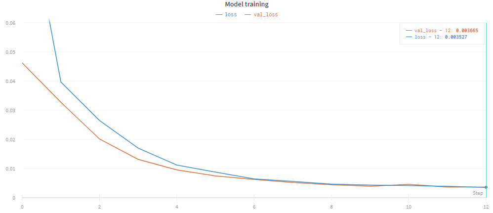
Training results
- 10k records made on the randomly generated track
- 12 epochs, 21m 45s on an RTX 2060
- The final validation loss was 0.003665.
Preview
Behavioural subnetwork
The architecture
Implementation
# New input layer
behaviourInput = Input(shape=(numberOfBehaviourInputs,), name="behaviourInput")

# ConvNet parts ...

# Behavioural net
z = behaviourInput
z = Dense(numberOfBehaviourInputs * 2, activation='relu')(z)
z = Dense(numberOfBehaviourInputs * 2, activation='relu')(z)
z = Dense(numberOfBehaviourInputs * 2, activation='relu')(z)

# Concatenating the convolutional networks with the behavioural network
o = Concatenate(axis=1)([z, c])
o = Dense(100, activation='relu')(o)
o = Dense(50, activation='relu')(o)

# Output layers ...

# Update the model inputs
model = Model(inputs=[imageInput, laneInput, behaviourInput], outputs=[steering_out, throttle_out])
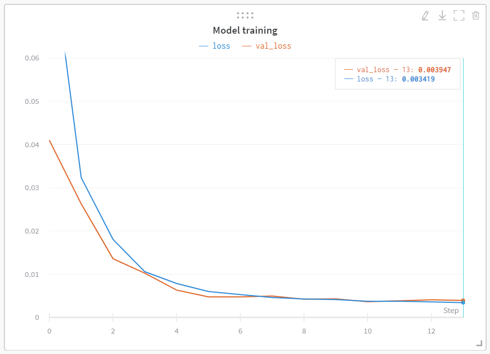
Training
- 7k records with approx. 20 lane changes
- Final validation loss: 0.003947
Preview
Further avenues
Advanced lane finding with object recognition
Advanced object recognition
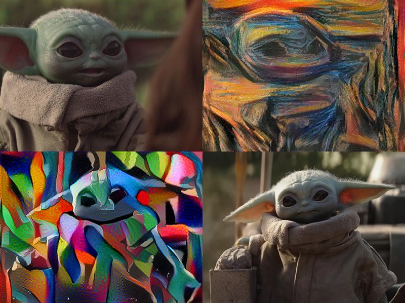
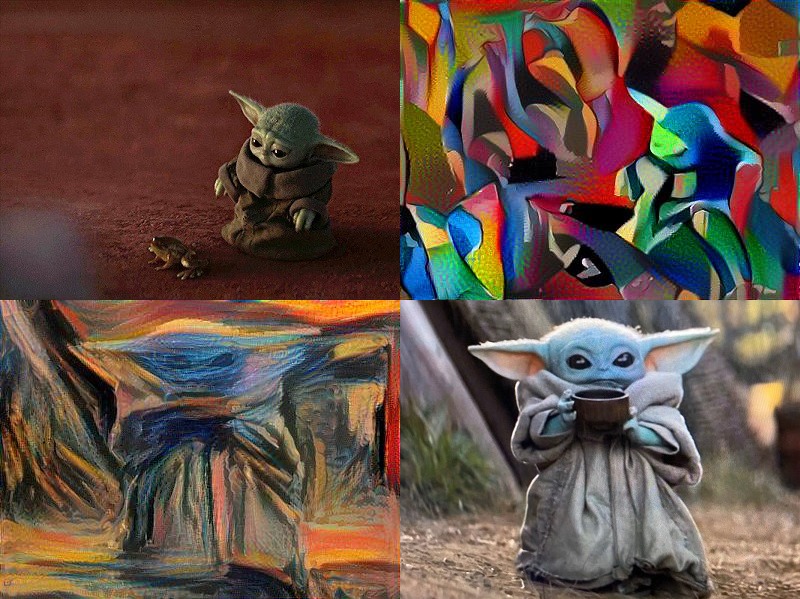
Data augmentation via neural art style transfer
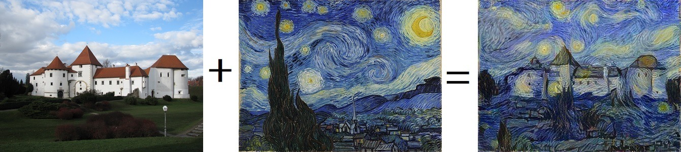
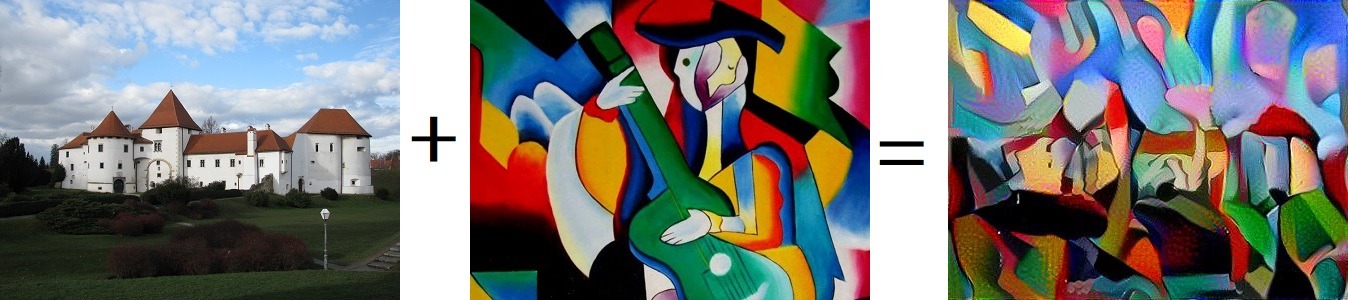
Data augmentation via neural art style transfer